Linear regression is a basic statistical tool that pretty much anyone who has worked with data is familiar with. In this post, I’m going to discuss some of the math and ideas behind the Bayesian approach, and try to do so in a way that will be easy to engage with for someone with a more traditional frequentist background.
Given n observations and d features per observation, my independent variable can be represented by a $n \times d$ matrix:
\[\bar X = [ X_1, X_2, ..., X_n]\] \[X_i = \begin{bmatrix}x_1\\x_2\\...\\x_d\end{bmatrix}\]The general linear model can be defined as:
\[y_i=\beta_0+\beta_1x_{i1}+\beta_2x_{i2} + … + \beta_dx_{id}+ϵ_i\]This can also be represented in a probabilistic form:
\[\mu_i=\beta_0+\beta_1x_{i1}+\beta_2x_{i2} + … + \beta_dx_{id}\] \[y_i ∼ \mathcal{N}(\mu_i,σ)\]This means that the values for the dependent variable $y_i$ are drawn from a normal distribution, paramaterized by its mean and standard deviation, where the mean is a linear function of X, itself paramaterized by $\beta_0, \beta_1 …, \beta_d$.
The goal of the classical (oft-called frequentist) approach is to find a way to choose values for these parameters that will maximize the likelihood of your data. This, sensibly enough, is called Maximum Likelihood Estimation (MLE). I can formulate this as:
\[\DeclareMathOperator*{\argmax}{arg\,max}\argmax_{\mu_i,σ}\prod_{i=1}^n \mathcal{N} (y_i ; \mu_i,σ)\]where $\mathcal{N}$ is the probability density function of the normal distribution on all of $y_i$. By multiplying the probability across all samples, I can find the joint probability of the data. Then by maximizing these paramaters I can find the parameter values that make observing this particular configuration of data most likely. That is to say that the probability of observing my data is most likely under a Gaussian characterized by these paramaters compared to all other possible paramaterizations.
In the Bayesian approach, my goal is no longer to estimate single values for these paramaters. It is instead to use Bayes rule to describe the distribution from which these parameters are drawn. I am no longer asking the question “which values for these paramaters make this configuration of my data most likely?” but instead, “what can I say about the possible values for these parameters, given this data the I have?”. We’re interested in the posterior, given the likelihood and our priors.
\[\underbrace{f(\mu_i,\sigma\mid Y,X)}_{\color{red}{\text{posterior}}} \propto \underbrace{\prod_{i=1}^n \mathcal{N}(y_i\mid \mu_i, \sigma)}_{\text{likelihood}} \; \underbrace{f_{\mu}(\mu) \, f_{\sigma}(\sigma)}_{\text{priors}}\]In the interest of keeping this post simple for now, I will gloss over some of the details of how we solve for the posterior. Suffice it to say it’s a hard problem due to an intractable integral, and for the purposes of this post we will be getting around this with variational inference, where we approximate the posterior by iteratively reducing it’s divergence from a different variational distribution, chosen from a limited family of distributions, described by some variational paramaters V. The other method is to use Markov-Chain Monte-Carlo (MCMC) techniques to create a graph such that a random-walk eventually converges to a stationary distribution that approximates the posterior.
Let’s look at some simple test cases and see how our results differ. Let’s start with the toy example where I have just 3, 1-dimensional data points $X=[0,3,4]$ and $Y=[1,6,10]$. Here are two plots: the left shows 5 samples from the posterior distibutions for the regression coefficients calculated with certain assumptions, and the right shows maximum likelihood estimation (under the assumption of normally distributed errors).
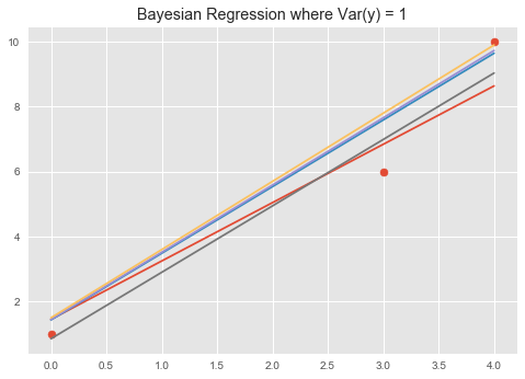
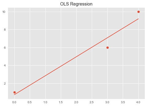
Hopefully unsuprisingly, these graphs look pretty similar - although it probably seems rather less useful to have 5 different random lines instead of 1. And if we look at the mean-squared error, the classical ordinary-least-squares approach actually has lower error! Why would you ever want to use the Bayesian approach instead? Let’s take a look at these visualizations of 10,000 samples from the posterior distribution for the coeffecients for the slope & intercept.
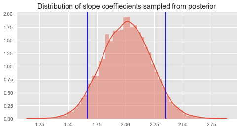
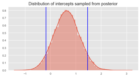
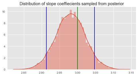
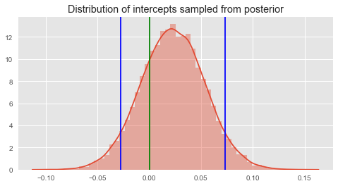
The vertical blue lines mark the 5th and 95th percentiles of the sample - that is, the range I can say with 90% confidence that the true values of my parameters fall. In the Bayesian world, these are known as credible intervals and are contrast to confidence intervals the frequentist approach uses - although again they are really asking totally different questions. But in my opinion, the Bayesian question is generally the one you actually intended to ask, and it provides an easy to understand range of uncertainty that doesn’t require imagining the results of hundreds of unperformed experiments.
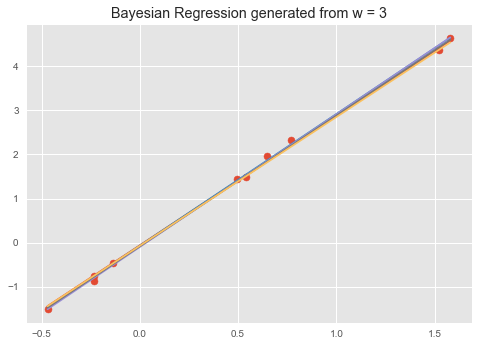
Let’s take a look at another example - in this case I’ve generated some data from a linear model + noise - the fit is graphed the same as above, but now on the posterior graph I’ve included a green line showing the true value of the generating parameter.
Here are the same graphs, generated from only 10 samples:
And now with 1,000 samples:
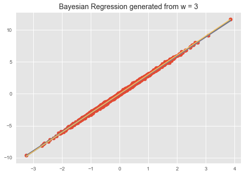
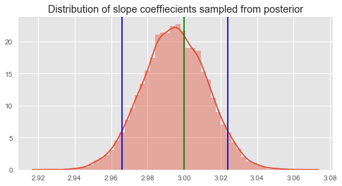
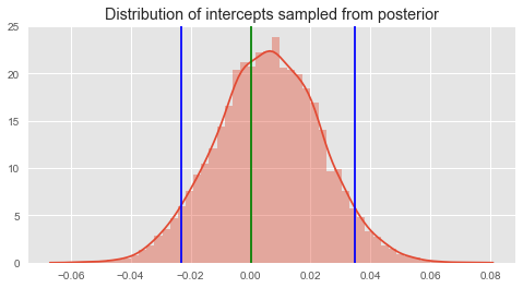
You can see a narrowing of the credible intervals that reflects the fact that our degree of certainty increases as the size of the sample does, which is what you would expect. [Note: I initially had an incorrect value for variance on the prior of the intercept - this resulted in the true value falling outside the range in the 10 sample case, but not the 1,000 sample case - this is because as we see more data, our prior becomes less important to the model.]
That’s all I’ll write in this post for now, but I’m working on an interface that will allow the user to adjust the sample size, priors, effect, etc. and see the results easily for themselves. I think increasing the accesibility of Bayesian tools to those who don’t need to grasp the math behind the inference stage is something that is very important, and can have a large impact on how stats are done across the social sciences. To this end, this post is a first exploratory step in writing a wrapper for parts of Edward to make it more neophyte friendly.